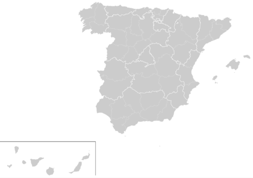
Spain map with D3

Since we will manage files and dependencies we choose Flask for a quick example. Any other framework could be used, it only consist on importing correctly all libraries.
The libraries used are the following:
Jquery: Common library used almost for anything. (Desc)
Jquery UI: Visual extension for Jquery (Desc, in this case used to create the time slider. We also add another extension (Ui slider pips) to this slider to customize even more.
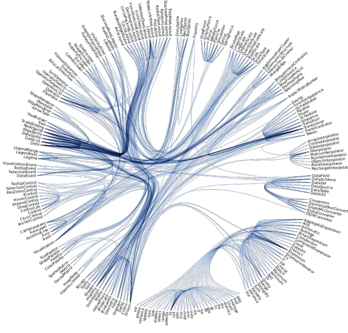
D3: D3.js is a JavaScript library for manipulating documents based on data. D3 helps you bring data to life using HTML, SVG, and CSS. In this case we use to create a map of Spain. More examples of D3 here.
D3 composite: Extension of D3 that allow to create proyections of maps. For example, in the case of Spain since the canary islands are far away from the peninsula, only using D3 we have a really off center map. This library also provides Spain provinces limits . Important: This library only works with the current set of Jquery and D3 version, if you want to use other versions, check the docs page.